Top Inventory Forecasting Models: MA, ES, ARIMA & When to Use Them

Inventory forecasting isn’t just about estimating future demand—it’s about choosing the right forecasting model to match your business's complexity, product behavior, and risk tolerance. From stable demand curves to erratic seasonal spikes or long-tail SKUs, no single model fits all scenarios.

This guide breaks down the most widely used inventory forecasting models—including Moving Average (MA), Exponential Smoothing (ES), ARIMA, and Croston’s Method—explaining how they work, when to use them, and where each one excels or fails. 

Whether you're managing thousands of SKUs in retail or planning production runs in manufacturing, understanding these models will help you make smarter, data-driven decisions that reduce overstock, prevent stockouts, and improve your supply chain efficiency

‍

Why Choosing the Right Inventory Forecasting Model Matters

Accurate inventory forecasting is critical for balancing supply and demand, minimizing carrying costs, and preventing both overstock and stockouts. But the accuracy of your forecast depends heavily on the model you choose—and not all models are suited to all demand patterns.

For example, a simple moving average may work well for products with stable, predictable sales, but it will fail in the presence of seasonal demand spikes or sudden shifts in consumer behavior. 

Conversely, advanced models like ARIMA or exponential smoothing can adapt to trends and volatility, but require clean data and statistical rigor. Choosing the wrong model doesn’t just lead to poor forecasts—it can result in lost revenue, excess inventory, higher logistics costs, and even broken customer trust.

The right forecasting model allows businesses to:

• Forecast demand at SKU or category level
• Improve replenishment accuracy
• Reduce manual planning and decision fatigue
• React quickly to changing demand patterns

Ultimately, selecting the appropriate inventory forecasting method is not a technical decision alone—it’s a strategic one that affects profitability, efficiency, and competitiveness.

‍

The Top Inventory Forecasting Models (And How They Work)

Choosing the right inventory forecasting model can make the difference between consistently meeting demand and constantly firefighting stockouts or overstock. Below are the most widely used forecasting models—explained in depth—so you can select the right one for your products, channels, and variability levels.

1. Moving Average (MA) Model

What It Is:
The Moving Average (MA) model smooths out demand fluctuations by calculating the average of demand over a fixed number of past periods. As each new period is added, the oldest one is dropped, hence the “moving” aspect. The idea is to filter out noise and identify a central demand trend over time.

When to Use:
Best for stable, linear demand patterns without strong seasonality or trend. Works well for fast-moving SKUs where demand doesn’t vary significantly month over month.

Pros:

• Very easy to implement and understand
• Requires minimal computational resources
• Good for short-term forecasts in consistent environments

Cons:

• Ignores recent changes in demand behavior
• Doesn’t respond well to trend or seasonal variations
• Requires manual adjustment of period window (e.g., 3-month vs 6-month MA)

Example:
If the last four months’ demand is [100, 120, 110, 130], a 4-period MA forecast is (100+120+110+130)/4 = 115 units for the next period.

‍

2. Exponential Smoothing (ES)

What It Is:
Exponential Smoothing is a weighted moving average technique that applies exponentially decreasing weights to older observations. Unlike MA, it emphasizes the most recent demand, making it more adaptive to changes in demand patterns. It comes in three major forms:

• Single ES: For level demand with no trend or seasonality
• Double ES (Holt’s Method): Accounts for trend by adding a second smoothing equation
• Triple ES (Holt-Winters): Adds seasonality adjustment for recurring patterns

When to Use:
Ideal for moderately variable demand with clear level, trend, or seasonal components. Works well for SKUs with promotional cycles, weather-sensitive products, or fashion seasonality.

Pros:

• More responsive than MA to recent demand shifts
• Suitable for short- and medium-term planning
• Can model both trend and seasonality

Cons:

• Requires parameter tuning (α, β, γ)
• Sensitive to noisy data if smoothing factors are not optimized
• Doesn’t perform well for erratic or intermittent demand

Example:
For a single exponential smoothing with α = 0.2 and last actual demand of 120 and previous forecast of 110:
New forecast = (0.2 × 120) + (0.8 × 110) = 112 units.

‍

3. ARIMA (AutoRegressive Integrated Moving Average)

What It Is:
ARIMA is a robust time series forecasting model that combines three components:

• AR (AutoRegressive): Uses past values to predict future ones
• I (Integrated): Applies differencing to make the series stationary (removing trend)
• MA (Moving Average): Models the error of previous predictions

When extended to handle seasonality, it becomes SARIMA (Seasonal ARIMA), which includes seasonal lags and differencing.

When to Use:
Useful for SKUs with strong autocorrelation or consistent patterns over time—such as monthly demand cycles, macroeconomic influence, or high-volume seasonal products.

Pros:

• Captures trend, seasonality, and noise in one unified model
• Highly customizable for different time-series behaviors
• Suitable for long-term forecasting with sufficient historical data

Cons:

• Requires stationary data (often involves preprocessing)
• Complex to configure (p, d, q) and evaluate (AIC/BIC criteria)
• Less interpretable for business users without statistical background

Example:
An ARIMA(1,1,1) uses 1 autoregressive term, 1 differencing term, and 1 moving average term. SARIMA(1,1,1)(1,0,1)[12] adds seasonal components with a cycle length of 12 (e.g., months in a year).

‍

4. Croston’s Method (for Intermittent Demand)

What It Is:
Croston’s method is specifically designed for SKUs with intermittent demand—that is, items that have many periods of zero sales followed by irregular spikes. It separately forecasts two things.

1. The average size of demand when it occurs
2. The average interval between demand events

By treating these two dimensions independently, it avoids the distortion that MA or ES would create for low-volume or sporadic items.

When to Use:
Perfect for spare parts, industrial components, and long-tail SKUs in eCommerce or B2B—where demand is unpredictable and infrequent.

Pros:

• Much more accurate than MA/ES for intermittent demand
• Reduces inventory holding costs for rarely sold items
• Helps in planning safety stock for slow-movers

Cons:

• Doesn’t handle trend or seasonality
• Assumes independence between demand size and interval
• Can be less accurate when demand intervals vary widely

Example:
If a spare part is ordered every 3 months in quantities of 15, Croston’s method treats that as two variables: 15 units (demand size) and 3 months (interval), forecasting future orders as a function of both.

‍

5. Machine Learning Models (Advanced Use Cases)

What It Is:
Machine learning (ML) models use algorithms to learn complex patterns from past data—going beyond historical sales to incorporate additional signals like price changes, promotions, weather, online behavior, regional factors, and even competitor pricing. Popular models include:

• Linear and Ridge Regression
• Random Forests & XGBoost
• Neural Networks (e.g., LSTM for time series)

When to Use:
ML forecasting is ideal for large-scale operations with high data maturity—especially when external factors strongly influence demand. Examples include multi-location retail, seasonal products with price sensitivity, or omnichannel inventory strategies.

Pros:

• Can capture non-linear relationships
• Highly accurate when trained on rich datasets
• Supports real-time forecasting with dynamic input variables

Cons:

• Requires significant historical and contextual data
• Needs data preprocessing and feature engineering
• Model transparency can be limited (black-box problem)

Example:
A Random Forest model could use features like last 3 months' sales, marketing spend, weather, product price, and competitor discounts to predict demand for a particular SKU.

‍

How to Choose the Right Inventory Forecasting Model

No single inventory forecasting model fits all businesses, product categories, or demand patterns. Choosing the right model requires evaluating your data maturity, operational complexity, SKU behavior, and forecasting horizon. Below are the core factors that help you determine the best-fit model for your inventory planning strategy.

1. Nature of Demand (Stable, Trend, Seasonal, Intermittent)

The first step is analyzing your demand pattern:

• If your demand is stable and linear, simple models like Moving Average may suffice.
• If you see seasonal peaks or upward/downward trends, use Exponential Smoothing (ES) or ARIMA variants.
• For irregular, low-frequency demand, such as spare parts or slow-moving SKUs, Croston’s Method is far more accurate.

Understanding your demand type helps eliminate models that would overreact or underreact to real-world changes.

‍

2. Volume and Velocity of SKUs

High-volume SKUs often benefit from more dynamic models (like ES or ARIMA) that can respond to fast changes in trend or stock-outs. Low-velocity SKUs, on the other hand, are better served with models that handle sparse data—such as Croston’s or heuristic-based reorder rules.

‍

3. Data Availability and Quality

• Simple models like MA or Single ES need only historical sales data.
• Advanced models (ARIMA, ML) require longer time-series data and, ideally, auxiliary variables like weather, price changes, promotions, or location data.
• If your dataset is limited or noisy, start with simpler models and evolve as your data improves.

‍

4. Forecasting Horizon

• For short-term planning (weeks to a few months), MA and ES offer enough responsiveness.
• For long-term strategic forecasting (quarters or seasons), ARIMA or ML models can provide better performance, especially when accounting for external demand drivers.

‍

5. Business Resources and Technical Capacity

• If your team has limited analytical resources, models like MA and ES can be implemented quickly in Excel or lightweight tools.
• If you have a dedicated data team or use advanced ERP/forecasting software, models like ARIMA, SARIMA, or machine learning algorithms become viable options.
• Consider ongoing maintenance: complex models often need retraining, hyperparameter tuning, and performance monitoring.

‍

6. Integration with Replenishment Systems

Your forecasting model must connect seamlessly with your inventory and ordering systems. It should drive actionable outcomes—like purchase order generation, safety stock buffers, or replenishment alerts—not just predictions.

Pro Tip:
Start simple. Many brands find success using hybrid approaches:

• Use MA or ES for high-volume, stable products
• Layer in ARIMA for trend-sensitive SKUs
• Apply Croston to long-tail inventory
• Adopt ML forecasting where product behavior depends on external inputs like promotions or weather

‍

EasyReplenish: Inventory Forecasting Software That Supports MA, ES, ARIMA & More

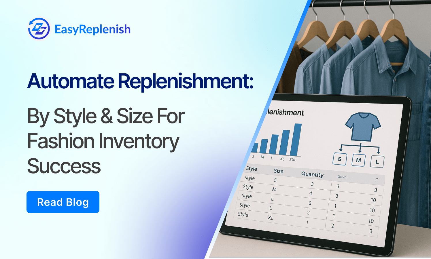
Choosing the right model is only one part of the equation—the bigger challenge is operationalizing it at scale across thousands of SKUs and dynamic demand environments. That’s where EasyReplenish helps. Built specifically for inventory-heavy businesses, EasyReplenish enables accurate, model-driven forecasting that directly powers smarter replenishment decisions.

1. Model-Backed Forecasting, Built In

EasyReplenish offers built-in support for key forecasting models including:

• Moving Average for simple, stable SKUs
• Single, Double, and Triple Exponential Smoothing for products with level, trend, or seasonal patterns
• ARIMA & SARIMA for complex time series forecasting
• Croston’s Method for intermittent and low-velocity items

Users can configure model preferences at the SKU or category level—or let EasyReplenish dynamically choose the best-fit model based on historical performance, variability, and demand patterns.

‍

2. Real-Time, Automated Forecasting

EasyReplenish integrates historical sales data, lead times, inventory position, and seasonality to generate real-time forecasts. As demand shifts, forecasts auto-adjust—triggering replenishment alerts or purchase orders before stockouts occur.

‍

3. No-Code Interface with Deep Customization

Whether you’re a planner, operations lead, or demand analyst, EasyReplenish offers:

• Configurable forecast horizons (weekly, monthly, seasonal)
• Custom smoothing parameters and model overrides
• Visual tools to compare forecast vs. actual demand
• Rule-based replenishment driven by forecast outputs

‍

4. Scalability Across Channels and Locations

For brands selling through multiple channels—DTC, retail, wholesale, or marketplaces—EasyReplenish supports location-level forecasting and allocation, ensuring optimal stock positioning across warehouses, stores, and fulfillment nodes.

‍

5. Built for Growth

Whether you're just transitioning from spreadsheets or managing millions in monthly inventory turnover, EasyReplenish gives you the forecasting depth of an enterprise tool—without the complexity.

‍

FAQs

Q1. What is the best inventory forecasting model for seasonal demand?

For products with strong seasonal patterns—such as fashion collections, holiday inventory, or weather-driven items—the most effective models are Triple Exponential Smoothing (Holt-Winters) or SARIMA. These models account for repeating seasonal fluctuations while also adjusting for trend and base demand. Simpler models like moving average or single smoothing often fail to capture these patterns accurately.

‍

Q2. How do I choose between Moving Average and Exponential Smoothing?

Moving Average (MA) is easier to implement but treats all historical data equally, making it slow to react to recent changes. Exponential Smoothing (ES) gives more weight to recent demand, making it more responsive and better suited for products with moderate variability. If demand is relatively flat, MA is sufficient. For more dynamic environments, ES typically delivers more accurate forecasts.

‍

Q3. Can ARIMA be used for inventory forecasting in retail?

Yes, ARIMA (AutoRegressive Integrated Moving Average) is widely used in retail and eCommerce to forecast SKU-level or category-level demand. It's particularly useful when demand shows trends, cycles, or autocorrelation. However, ARIMA models require clean, stationary data and technical expertise for setup, so they’re best suited for businesses with established analytics workflows or forecasting software like EasyReplenish.

‍

Q4. What is the best model for forecasting intermittent or slow-moving SKUs?

For products with sporadic or unpredictable demand—such as spare parts or long-tail eCommerce items—Croston’s Method is the preferred forecasting model. It separately forecasts the demand size and interval between orders, outperforming standard MA or ES techniques for low-volume items with zero-demand periods.

‍

Q5. Does EasyReplenish support automatic selection of forecasting models?

Yes. EasyReplenish can automatically select the most suitable forecasting model for each SKU or category based on demand history, product velocity, and variability. It supports MA, ES, ARIMA, and Croston’s methods—allowing businesses to scale model-based forecasting without needing in-house statistical expertise. You can also manually override models or adjust parameters when needed.