The Real Reason Replenishment Breaks

Replenishment only works when its parameters are set correctly. Lead time, EOQ, and min–max levels control when the system reorders and how much it orders—and even small inaccuracies in these values create stockouts, excess stock, or erratic order patterns.

Most brands don’t struggle with forecasting; they struggle because their parameters are either outdated, assumed, or applied uniformly across all SKUs. This guide explains how to set replenishment parameters with precision, how to adjust them for different SKU behaviors, and how to keep them aligned with real-world demand and supplier performance.

Before You Set Parameters — Identify the Replenishment Archetype of Each SKU

Replenishment parameters only work when they’re aligned to the behaviour of the SKU. Setting the same lead time buffer, EOQ logic, or min–max range for all products is the fastest way to break availability. Start by classifying SKUs into four replenishment archetypes—each requiring a different parameter strategy.

1. Stable & High-Velocity SKUs (Continuous Replenishment)

These SKUs have predictable, steady sales with minimal volatility.

Parameter implication:

• Lead times can be tight; buffers can be low.
• Min levels should stay close to actual consumption.
• EOQ and Max levels can be optimized for cost and space.

These items benefit most from automated, high-frequency replenishment.

2. Medium Velocity SKUs With Demand Variability

Sales are consistent but prone to spikes or short-term shifts.

Parameter implication:

• Lead time buffers must absorb volatility.
• Min levels require a volatility factor rather than pure consumption logic.
• Max levels should align with forecasted peaks or promotional cycles.

These SKUs need more conservative parameters to avoid mid-cycle stockouts.

3. Long-Tail / Low-Risk SKUs

Low or intermittent demand, often service-level driven, not revenue-driven.

Parameter implication:

• EOQ and MOQ constraints matter more than demand.
• Min levels can be set higher relative to sales to avoid stockouts from sporadic orders.
• Max levels should stay tightly controlled to prevent dead stock.

These SKUs are replenished infrequently, so parameter precision prevents accumulation.

4. Size–Color Matrix SKUs (Fashion)

Demand varies at the size–color level, not at style level.

Parameter implication:

• Parameters must be size-level: Min–Max at “SKU × size × color.”
• Lead time buffers must reflect vendor unpredictability and season timelines.
• Max levels should follow size curves, not total style forecasts.

This is the only segment where parameter granularity determines availability.

Setting Lead Time — Operational Rules for Accuracy

Lead time is the most sensitive replenishment parameter. If it’s wrong—by even a few days—your entire min–max logic collapses. Instead of relying on vendor-stated lead times or last month’s numbers, use these operational rules to set lead time accurately.

1. Use System-Observed Lead Time, Not Vendor Promises

Always take GRN-to-PO data from your system across a rolling window (6–12 weeks).

Rule: The vendor’s declared lead time is a reference; the system’s actual lead time is the truth.

2. Identify Lead Time Variability, Not Just the Average

Variance matters more than the mean. A vendor with a 10-day average and ±4 days’ deviation needs a different buffer than one with a stable 12-day lead time.

Rule: Lead time = average + variability buffer.

3. Set Lead Time Separately for Each SKU–Vendor Pair

Lead time is not vendor-wide. Different SKUs from the same vendor often have different production or packing timelines.

Rule: Lead time granularity must match SKU behaviour, not vendor convenience.

4. Increase Lead Time Buffers During Seasonal or Operational Stress

Peak season, festive periods, port congestion, and production overload push lead times up.

Rule: Apply seasonal lead time multipliers for periods where delays are predictable.

5. Keep Lead Time Location-Specific in Multi-Warehouse Environments

Inbound times differ between DCs, stores, and regional warehouses.

Rule: Do not use a global lead time; set lead times per location.

6. Override Lead Time Temporarily When Reality Changes

Vendor changeovers, material shortages, QC issues, or transport disruptions require immediate parameter overrides.

Rule: Lead time overrides should be part of weekly replenishment governance.

7. Review Lead Time Weekly for High-Velocity SKUs and Monthly for Others

Fast movers are most sensitive to lead time errors; long-tail SKUs can be reviewed less frequently.

Rule: Lead time review cadence must follow SKU velocity.

‍

Setting EOQ — Choosing Practical Order Quantities

EOQ is useful only when it reflects operational reality. Most brands misapply it because they treat EOQ as a formula instead of a decision framework. The goal is not to find the “ideal” order quantity—it’s to find the most efficient one based on demand patterns, vendor constraints, and cash cycles.

1. Use EOQ Only for Stable, Predictable SKUs

EOQ works when demand is consistent and the SKU is always replenished.

Rule: Apply EOQ to steady movers; avoid it for seasonal, fashion, or high-volatility items where demand shifts quickly.

2. Always Compare EOQ With MOQ, Carton Size & Volume Breaks

Real-world ordering is rarely continuous; vendors impose constraints.

Rule: EOQ is a baseline. The final order quantity is:
max(EOQ, MOQ, vendor carton multiples).

3. Increase EOQ for High-Margin, Fast-Moving SKUs

The holding cost impact is low, and stockouts hurt more than carrying extra units.

Rule: For high-velocity winners, push EOQ upward to avoid frequent ordering.

4. Reduce EOQ for Long-Tail or Slow-Moving SKUs

These SKUs risk dead stock if ordered in bulk.

Rule: Keep EOQ conservative—match demand closely and avoid large batches.

5. Adjust EOQ Based on Cashflow and Purchase Cycles

Many brands ignore working capital cycles, and EOQ becomes misaligned.

Rule: If cashflow is tight, allow EOQ to drop; prioritize availability, not bulk optimization.

6. Modify EOQ for Inbound Logistics Efficiency

Shipping from overseas? Ordering full pallets or containers?

Rule: Align EOQ with freight optimization—not just per-SKU economics.

7. Review EOQ Quarterly or When Vendor Costs Change

Ordering cost, holding cost, and purchase price shift regularly.

Rule: EOQ must be recalculated when cost structures change; otherwise, it becomes obsolete

‍

Setting Min–Max Levels — The Parameters That Actually Control Availability

Min–Max is where replenishment succeeds or fails. Lead time and EOQ matter, but Min–Max determines the system’s day-to-day ordering behaviour. These values must reflect demand patterns, SKU importance, variability, and operational constraints—not just theoretical calculations.

1. Set the Min Level Based on Demand Risk, Not Just Consumption

Min shouldn’t be blindly tied to average demand during lead time. Instead, it should reflect how risky the SKU is to run out of.

Rule:

• Stable SKUs → Min close to actual lead-time demand
• Variable SKUs → Min inflated by a volatility factor
• Long-tail → Min slightly above typical order size to avoid single-order stockouts
• Fashion → Min set at size level, not style level

2. Set the Max Level to Control Inventory Exposure

Max defines how much stock the system pulls in once Min is breached. It should never be a random multiple.

Rule:
Use Max to balance:

• Order quantity constraints (MOQ, carton size)
• Space capacity
• Seasonality and expected peaks
• Cashflow limits

For fast movers, Max should comfortably cover the full review cycle plus buffer. For slow movers, Max should be tightly restricted to avoid accumulation.

3. Align Min–Max With the SKU’s Replenishment Archetype

Each SKU type behaves differently; parameters must follow.

Rule:

• High-velocity → Narrow Min–Max band, frequent small orders
• Medium velocity → Wider band to absorb variability
• Long-tail → Low Max, higher relative Min
• Fashion → Min–Max tailored to size curves and style–season windows

4. Expand Min–Max During Season Peaks; Tighten During Troughs

Demand doesn’t stay flat across the year.

Rule:
Create seasonal Min–Max adjustments:

• Pre-season: increase Max
• Mid-season: increase Min to protect availability
• End of season: reduce Max to prevent leftover stock

5. Review Min–Max More Frequently for High-Impact SKUs

Static Min–Max levels break as soon as demand or lead time shifts.

Rule:

• High-velocity SKUs → Weekly review
• Mid-velocity → Monthly
• Long-tail → Quarterly

This keeps parameters aligned with real-world consumption.

6. Use Min–Max Overrides When Reality Changes

System rules cannot predict disruptions.

Rule:
Override Min–Max temporarily if:

• Vendor delays increase lead time
• A promotion or event drives short-term demand
• QC holds or inbound delays shrink available stock
• A size or variant sells disproportionately faster

This prevents stockouts during anomalies.

The Parameter Setting Framework Used by High-Performing Brands

Replenishment parameters work only when they are aligned and updated consistently. The most effective brands follow a structured workflow that links SKU behaviour, demand variability, vendor performance, and operational constraints into one unified parameter-setting process.

1. Classify SKUs by Velocity and Variability

Parameter setting starts with categorization.

Rule: Assign each SKU to an archetype (stable, variable, long-tail, fashion matrix). This defines how aggressive or conservative each parameter must be.

2. Set Lead Time Using System Data + Variability Buffer

Lead time becomes the anchor for all downstream parameters.

Rule: Use system-observed lead time, add variability, and adjust for seasonal or operational conditions.

3. Choose the Ordering Logic (EOQ, MOQ, or Volume-Based)

Decide how the brand prefers to order for each SKU type.

Rule:

• Stable SKUs → EOQ or MOQ-based
• Variable SKUs → MOQ or demand-driven quantity
• Long-tail → smallest economic quantity
• Fashion → size-level ordering aligned to the ratio curve

4. Set Min Levels to Cover Lead-Time Demand + Risk

Min defines when the system reorders.

Rule: Min follows the SKU’s volatility level, not just the lead-time consumption.
Stable SKUs get tight Mins; volatile and long-tail SKUs get higher Mins.

5. Set Max Levels to Control Inventory Exposure

Max defines how much inventory the system pulls in.

Rule: Max reflects order constraints, seasonality, space, and cash.
It must be high enough to avoid multiple POs but low enough to avoid overstock.

6. Define Review Cadence by SKU Importance

Parameters must shift with demand, vendor performance, and seasonality.

Rule:

• High-velocity → Weekly review
• Mid-velocity → Monthly
• Low-velocity → Quarterly
• Fashion → Seasonal pre/mid/end reviews

7. Use Exceptions and Overrides When Reality Changes

This is where top-performing brands differentiate themselves.

Rule: Whenever lead time jumps, demand spikes, a promotion activates, or a size sells disproportionately, override parameters instead of waiting for the next cycle. Real-world replenishement requires dynamic adjustments.

Outcome: A Replenishment System That Reacts to Reality, Not Assumptions

Following this framework ensures that lead time, EOQ, and Min–Max work together—driving clean, stable replenishment with fewer stockouts and fewer unnecessary orders.

‍

Advanced Parameter Tuning for Fashion, D2C & Multi-Category Brands

Fashion and D2C categories behave very differently from stable retail segments. Demand volatility, size–color dependencies, seasonal timelines, and rapid SKU churn require more dynamic parameter tuning. High-performing brands adjust Min–Max, lead time buffers, and ordering logic at a far more granular level.

1. Size-Level Min–Max Using Ratio Curves (Fashion Only)

Demand distribution across sizes rarely matches total style velocity.

Rule: Set Min–Max at the size × color level using historical size curves, not at style level. This keeps mid-selling sizes in stock even when the style sell-through is uneven.

2. Parameter Logic for Never-Out-of-Stock (NOS) Styles

NOS SKUs require tighter controls because stockouts directly impact revenue.

Rule:

• Min = higher coverage of lead-time demand
• Max = higher cushion during season peaks
• Lead time = monitored weekly, not monthly

NOS items get the most aggressive protection.

3. Seasonal Parameter Adjustments Before, During & After the Season

Fashion demand follows distinct phases.

Rule:

• Pre-season: Increase Max to support the launch window
• Mid-season: Raise Min to protect high-velocity sizes
• End-of-season: Reduce Max sharply to avoid carryover

This ensures availability early and minimizes leftover stock late.

4. Tuning Parameters for Short-Lifecycle SKUs (D2C Product Drops)

D2C brands launch rapid cycles with unpredictable demand.

Rule:Avoid EOQ. Use demand pacing + rapid Min–Max adjustments for the first 2–3 weeks post-launch until demand stabilizes. This reduces the risk of overcommitting too early.

5. Adjust Parameters for Multi-Channel or Multi-Location Selling

Demand behaves differently across online, retail, marketplace, and warehouse channels.

Rule: Set parameters separately per channel/location.

Online may need higher Mins for fast delivery promises; stores may need tighter Max to avoid crowding shelf space.

6. Handling SKUs With High Vendor Volatility

Fashion vendors often fluctuate in production cycle, quality checks, and delivery timelines.

Rule:
Increase lead time buffers for vendors with inconsistent past performance—even if their declared lead time is stable. This prevents last-minute stockouts caused by supplier unreliability.

7. Parameter Tuning for High-Margin vs Low-Margin Categories

Categories with very different margin profiles require different risk appetites.

Rule:

• High-margin categories → higher Max, higher buffer
• Low-margin categories → conservative Max, strict ordering

This balances cashflow with availability.

How Modern Tools Automate Parameter Setting (Without Becoming Promotional)

Modern inventory systems don’t replace planners—they remove the manual guesswork behind parameter maintenance. Instead of relying on fixed values that become outdated quickly, these tools monitor demand patterns, vendor behaviour, and stock movements continuously, and surface adjustments before issues appear.

1. Auto-Sensing Lead Time Changes

Lead times fluctuate far more than most teams realise. Modern systems track actual PO → GRN timelines and detect patterns such as:

• gradual vendor slowdown
• repeated delays for certain SKUs
• location-specific inbound differences

What automation does:
When average lead time changes or variability increases, the system updates the recommended lead time buffer or triggers a notification, ensuring parameters reflect current supplier performance—not outdated assumptions.

2. Auto-Adjusting Min–Max Based on Sales Velocity Shifts

Demand rarely stays flat. SKUs move through phases—launch spikes, mid-cycle stability, late-cycle tapering.

What automation does:
Tools detect velocity changes and adjust recommended Min–Max levels by:

• increasing Min when consumption rises
• decreasing Max when sell-through drops
• tightening Min–Max when demand stabilises

This prevents both mid-cycle stockouts and late-cycle overstock.

3. Automated Alerts When Parameters Break Reality

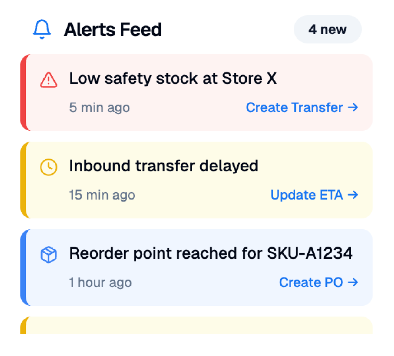
Even with automation, exceptions happen. High-performing systems monitor live conditions and raise alerts when parameters stop matching real-world behaviour.

Common triggers include:

Demand Spike

Sudden increases in sales outpace the current Min–Max range.
Alert: “Demand exceeded expected velocity—review Min level.”

Vendor Delay

Inbound shipments repeatedly miss planned receipt dates.
Alert: “Lead time deviation increasing—adjust lead time buffer.”

Stock Freeze or QC Hold

Inventory is physically present but unavailable for sale.
Alert: “Available stock below Min due to freeze—replenishment at risk.”

Wrong Min–Max Combination

System detects that Max cannot cover the review cycle or Min is too close to daily consumption.

Alert: “Parameter mismatch—recalculate Min–Max for SKU.”

Conclusion — Why Parameter Setting Must Be a Continuous Process, Not a One-Time Setup

Replenishment parameters only work when they evolve with the business. Lead times shift, demand patterns change, vendors fluctuate, and SKU behaviour moves through phases. If parameters stay static, the system starts operating on outdated assumptions—resulting in stockouts, excess stock, and erratic reordering.

High-performing brands treat parameter setting as a continuous process: weekly for critical SKUs, monthly for the rest, with overrides whenever real-world conditions change. When lead time, EOQ, and Min–Max are maintained as living inputs, replenishment becomes stable, predictable, and far less dependent on firefighting.

FAQs

1. How often should replenishment parameters be recalculated versus simply reviewed?

Recalculation is needed when cost structures, vendor performance, or demand patterns shift materially. Review is a check for alignment; recalculation is a reset. High-velocity SKUs may need recalculation monthly, while long-tail SKUs may only need it quarterly.

2. Should Min–Max levels be standardized across categories or set independently?

They must be set independently. Category behaviour—margins, demand cycles, vendor reliability, and SKU lifecycle—varies widely. Using a uniform Min–Max model across all categories almost always leads to excess in some areas and shortages in others.

3. What data quality issues most commonly distort replenishment parameters?

Inaccurate GRN dates, missing stock adjustments, unrecorded returns, and inconsistent sales timestamps are the biggest causes. If base data is unreliable, lead times, Min–Max ranges, and EOQ calculations lose accuracy regardless of methodology.

4. Can replenishment parameters be different for the same SKU across channels?

Yes, and they often should be. Online channels need higher Min levels for fast fulfillment, while physical stores may require restricted Max levels due to space constraints. Treating all channels identically usually misaligns inventory exposure.

5. How do promotions or planned spikes fit into replenishment parameters?

Promotions require temporary parameter overrides—not permanent changes. Adjust Min and Max upwards for the promotion period, but revert them once the spike passes. Long-term parameter shifts should not be based on short-term events.

6. When is it better to ignore EOQ entirely?

Ignore EOQ for short-lifecycle products, fashion drops, highly volatile items, and any SKU with unpredictable size or variant-level demand. In these cases, demand-driven or MOQ-based ordering performs substantially better than EOQ.

‍